TableDiffusion is a deep learning algorithm I developed for training diffusion models on tabular data under differential privacy guarantees.
The goal is to enable the synthesis of data that maintains the statistical properties of the original dataset while ensuring the privacy of individuals’ information. This is an extension of my Masters Thesis work. The most notable model from my research is TableDiffusion, the first differentially-private diffusion model for tabular data, which outperformed the pre-existing GAN-based approaches.
If the above embed doesn’t work, you can watch it directly on YouTube: https://youtu.be/2QRrGWoXOb4
Why synthesise tabular data?
ML is accelerating progress across fields and industries, but relies on accessible and high-quality training data. Some of the most important datasets are found in biomedical and financial domains in the form of spreadsheets and relational databases. But this tabular data is often sensitive in nature and made inaccessible by privacy regulations like GDPR, creating a major bottleneck to scientific research and real-world applications of AI.
Synthetic data generation is an emerging field that offers the potential to unlock sensitive data: by training ML models to represent the statistical structure of the dataset and synthesise new samples, without compromising individual privacy.
What’s the catch?
Generative models tend to memorise and regurgitate training data, which undermines the privacy goal.
To remedy this, researchers have incorporated the mathematical framework of Differential Privacy (DP) into the training process of neural networks, limiting memorisation and enforcing provable privacy guarantees. But this creates a trade-off between the quality and privacy of the resulting data.
The GAN is dead, long live the diffusion model
Generative Adversarial Networks (GANs) were the leading paradigm for synthesising tabular data under Differential Privacy, but suffer from unstable adversarial training and mode collapse. These effects are compounded by the added privacy constraints. The tabular data modality exacerbates this further, as mixed data types, non-Gaussian distributions, high-cardinality, and sparsity are all challenging for deep neural networks to represent and synthesise. Yet, it is precisely tabular data that is most likely to be sensitive and valuable to solving real-world problems.
My contributions
For my Masters thesis, I optimised the quality-privacy trade-off of generative models, producing higher quality tabular datasets with the same privacy guarantees.
- I first developed novel end-to-end models that leverage attention mechanisms to learn reversible representations of tabular data. Whilst effective at learning dense embeddings, the increased model size rapidly depletes the privacy budget.
- Next, I introduced TableDiffusion, the first differentially-private diffusion model for tabular data synthesis.
Awesome results
My experiments showed that TableDiffusion produces higher-fidelity synthetic datasets, avoids the mode collapse problem, and achieves state-of-the-art performance on privatised tabular data synthesis. By implementing TableDiffusion to predict the added noise, we enabled it to bypass the challenges of reconstructing mixed-type tabular data. Overall, the diffusion paradigm proves vastly more data and privacy efficient than the adversarial paradigm, due to augmented re-use of each data batch and a smoother iterative training process.
But why diffusion models?
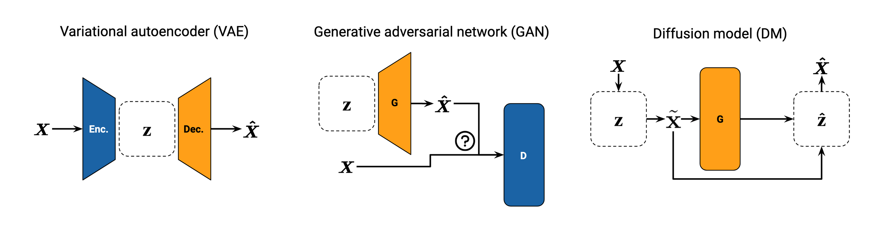
Unlike traditional generative models (GANs and VAEs) that learn the sampling function end-to-end, DMs define the sampling function through a sequential denoising process, which divides the task into many smaller and simpler steps, resulting in smoother and more stable training and simpler neural networks. But diffusion models remain unexplored in the domain of tabular data.
Notably, DMs can be implemented to predict the added Gaussian noise instead of directly denoising data. Outputting standard Gaussian noise is much easier for neural networks than outputting sparse, heterogeneous data with varying non-Gaussian distributions. This, along with the training robustness and parameter efficiency of diffusion models, makes them an ideal candidate for differentially-private tabular dataset synthesis.
I based my tabular diffusion models on the widely-validated and flexible formulation of DDPMs (Denoising Diffusion Probabilistic Models), which is based on two Markov chains:
- a forward chain that perturbs data to noise, and
- a reverse chain that converts noise back to data.
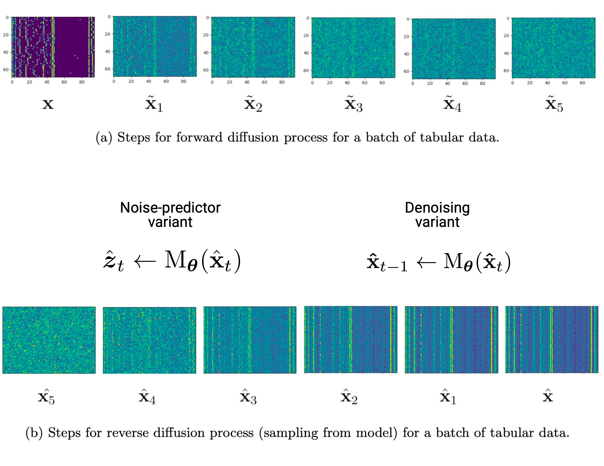
Forward process
In the forward process, we start with a batch of real data $\mathbf{x}$ and iteratively add increasing amounts of noise according to a scheduler. The simplest version of this would be sampling standard Gaussian noise $\boldsymbol{\xi} \sim \mathcal{N}(\boldsymbol{0}, \boldsymbol{I})$ and scaling it by $\sqrt{\beta_t}$ according to a linear schedule $\beta_t = \frac{t}{T}$, where $T$ is the total number of time steps and $t$ is the current step. In this case, the forward diffusion process can be expressed as:
$$\mathbf{x}_{t+1} = \mathbf{x}_{t} + \boldsymbol{z}_t$$where $\mathbf{x}_t$ is the batch of data at time step $t$ and $\boldsymbol{z}_t \sim \mathcal{N}(\boldsymbol{0}, \boldsymbol{I})\sqrt{\beta_t}$ is scaled Gaussian noise.
Reverse process
In the reverse process, we aim to denoise the data by going from the final time step $\mathbf{x}_T$, which is pure noise, back to the initial step $\mathbf{x}_0$, which approximates the real batch of data $\mathbf{x}$. We achieve this by training the parameters $\boldsymbol{\theta}$ of a neural network $M_{\boldsymbol{\theta}}$.
But we have three choices for designing the model’s objective function: predict the original data from the noised data (denoising), predict the added noise from the noised data (noise prediction), or predicting some score function of the noised data.
I implemented both denoising and noise-predicting DMs. The latter is more instructive, as it is unique to the diffusion paradigm. The model learns to predict the noise $\boldsymbol{z}_t$ added at each step:
$$\boldsymbol{z}_t \approx M_{\boldsymbol{\theta}}(\mathbf{x}_t)$$Given a prediction for $\boldsymbol{z}_t$, we can compute a prediction for $\mathbf{x}_{t-1}$:
$$\mathbf{x}_{t-1} \gets \mathbf{x}_t - M_{\boldsymbol{\theta}}(\mathbf{x}_t)$$By training the neural network in this way, we essentially learn to reverse the diffusion process and recover the original data from the noisy data. After training, the neural network can be used to generate new samples by applying the reverse process to a sample of pure noise.
Applying diffusion to tabular data
The majority of work on diffusion models has been done in the context of image data. In those contexts, autoencoders are often used to learn a compressed latent representation of the images and diffusion is performed in the latent space. In applying the diffusion paradigm to sensitive tabular data, I departed from prior work in a few notable ways:
- Firstly, instead of compressing an image to a latent space using an encoder network, I used a custom preprocessing approach to convert the mixed-type tabular data into a homogeneous vector representation and
- Secondly, in simplifying both diffusion processes by using only a few diffusion steps and by omitting the addition of noise between diffusion steps in the reverse process.
These modifications adapt the diffusion paradigm to the lower-dimensional manifolds of tabular data and performed better in our initial experiments, compared to the standard diffusion approaches for the image modality. Many aspects of standard diffusion implementations are unnecessary when training under DP-SGD, as the gradient clipping and noising serves to regularise the model and prevent overfitting.
Tabular data is lower dimensional than images, and our diffusion models are much smaller and more efficient (because they are optimised for the privacy-preserving context), so full sampling is fast. This allows us to simplify away many of these sophisticated techniques for our context.
The noise at each diffusion step $t$ is scaled by a variable $\beta_t$, which we draw from a cosine schedule:
$$\beta_t = \frac{1 - \cos\left(\frac{\pi t}{T}\right)}{2},$$where $T$ is the total number of diffusion steps and $t \in \{1, 2, \ldots, T\}$ is the current step. The noise schedule, through the scaling variable $\beta_t$, determines the magnitude of noise that is added at each step. At each step $t$, the noised data $\tilde{\mathbf{x}}_t$ is generated by adding Gaussian noise $\boldsymbol{\xi} \sim \mathcal{N}(\boldsymbol{0}, \boldsymbol{I})$ to the real data $\mathbf{x}$. The noise is scaled by $\beta_t$ as determined by the noise schedule:
$$\tilde{\mathbf{x}}_t = \mathbf{x} + \sqrt{\beta_t} \cdot \boldsymbol{\xi},$$Compared to earlier diffusion model work that used a linear noise schedule, adding noise more gradually through a cosine schedule reduces the number of forward process steps $T$ needed by an order of magnitude, whilst achieving similar sample quality.
We implemented two variants of the model, one which predicts the added noise and one which predicts the denoised data. This allowed for an ablation analysis of which diffusion properties affect synthetic data fidelity.
TableDiffusion model
The most notable model from my Thesis research is TableDiffusion, the first differentially-private diffusion model for tabular data.
The training process operates under differentially-private stochastic gradient descent (DP-SGD), providing provable privacy guarantees, whilst allowing arbitrary quantities of data to be synthesised from the same distribution as the training data.
TableDiffusion algorithms for training and sampling
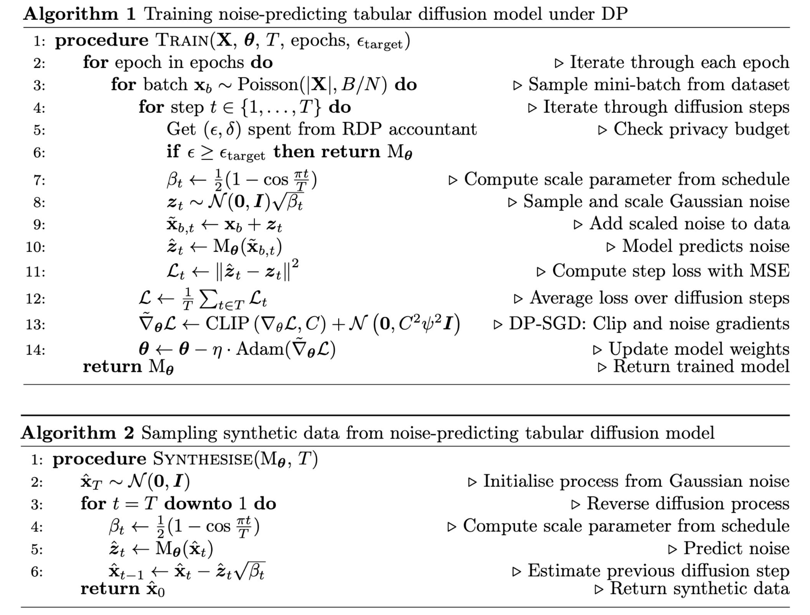
We can see that this algorithm is broadly similar to training a supervised neural network. We observe the same nested loops over epochs and batches of data (lines 2-3). Instead of sampling fixed-sized batches of data, we use Poisson sampling to get batches approximately $B$ in size (line 3). This sampling-based technique consumes the privacy budget slower than the deterministic batching commonly seen in gradient descent.
In the diffusion model, we also have an additional inner loop (line 4) over the steps $t \in \{1, \ldots, T\}$ in the forward diffusion process. This means that each batch of data is used $T$ times, augmented by varying levels of added noise. Unlike GAN-based and VAE-based models, this effectively gives the diffusion model $T$ times more data to learn from, without affecting the privacy budget. For each diffusion step $t$, the data is noised, the model predicts the noise, and the loss between the predicted and true noise is calculated (lines 9-11).
At the end of the diffusion loop, the losses for each step are aggregated (line 12). This is the point at which DP-SGD is implemented, clipping the gradients of the aggregated loss and adding further noise (line 13).
Finally, the privatised gradients are used to update the model parameters with the Adam optimiser (line 14). This is repeated for each batch sample and each epoch, until either the epoch limit (line 2) or the target privacy value $\epsilon_{\text{target}}$ is reached (line 6).
Once trained, we can sample synthetic data $\hat{\mathbf{x}}$ by sampling pure noise from a standard multivariate Gaussian of the same shape as the transformed data, then iteratively feeding it through the model in the reverse diffusion process, subtracting the (scaled) predicted noise at each step $t$.
Training code example (with Pytorch)
# Training loop
for epoch in range(n_epochs):
    self._elapsed_epochs += 1
    for i, X in enumerate(train_data):
        if i > 2 and loss.isnan():
            print("Loss is NaN. Early stopping.")
            return self
        self._elapsed_batches += 1
        real_X = Variable(X.type(Tensor))
        agg_loss = torch.Tensor([0]).to(self.device)

        # Diffusion process with cosine noise schedule
        for t in range(self.diffusion_steps):
            self._eps = self.privacy_engine.get_epsilon(self._delta)
            if self._eps >= self.epsilon_target:
                print(f"Privacy budget reached in epoch {epoch} (batch {i}, {t=}).")
                return self
            beta_t = get_beta(t, self.diffusion_steps)
            noise = torch.randn_like(real_X).to(self.device) * np.sqrt(beta_t)
            noised_data = real_X + noise

            if self.pred_noise:
                # Use the model as a diffusion noise predictor
                predicted_noise = self.model(noised_data)

                # Calculate loss between predicted and actualy noise using MSE
                numeric_loss = mse_loss(predicted_noise, noise)
                categorical_loss = torch.tensor(0.0)
                loss = numeric_loss

            else:
                # Use the model as a mixed-type denoiser
                denoised_data = self.model(noised_data)

                # Calculate numeric loss using MSE
                numeric_loss = mse_loss(
                    denoised_data[:, :categorical_start_idx],
                    real_X[:, :categorical_start_idx],
                )

                # Convert categoricals to log-space (to avoid underflow issue) and calculate KL loss for each original feature
                _idx = categorical_start_idx
                categorical_losses = []
                for _col, _cat_len in self.category_counts.items():
                    categorical_losses.append(
                        kl_loss(
                            torch.log(denoised_data[:, _idx : _idx + _cat_len]),
                            real_X[:, _idx : _idx + _cat_len],
                        )
                    )
                    _idx += _cat_len

                # Average categorical losses over total number of categories across all categorical features
                categorical_loss = (
                    sum(categorical_losses) / self.total_categories
                    if categorical_losses
                    else 0
                )

                loss = numeric_loss + categorical_loss

            # Add losses from each diffusion step
            agg_loss += loss

        # Average loss over diffusion steps
        loss = agg_loss / self.diffusion_steps
        print(f"Batches: {self._elapsed_batches}, {agg_loss=}")

        # Backward propagation and optimization step
        self.optim.zero_grad()
        loss.backward()
        self.optim.step()

return self
Sampling code example (with Pytorch)
def sample(self, n=None, post_process=True):
    self.model.eval()
    n = self.batch_size if n is None else n

    # Generate noise samples
    samples = torch.randn((n, self.data_dim)).to(self.device)
    fig, axs = plt.subplots(self.diffusion_steps, 4, figsize=(4*self.diffusion_steps, 4*4))

    # Generate synthetic data by runnin reverse diffusion process
    with torch.no_grad():
        for t in range(self.diffusion_steps -1, -1, -1):
            beta_t = get_beta(t, self.diffusion_steps)
            noise_scale = np.sqrt(beta_t)

            if self.pred_noise:
                # Repeatedly predict and subtract noise
                pred_noise = self.model(samples)
                predicted_noise = pred_noise * noise_scale
                samples = samples - predicted_noise
            else:
                # Repeatedly denoise
                samples = self.model(samples)

    synthetic_data = samples.detach().cpu().numpy()
    self.model.train()

    if not post_process:
        return synthetic_data

    # Postprocessing: apply inverse transformations
    # ...
    # Cast to the original datatypes for dataframe compatibility
    # ...

    return df_synthetic
More information
- Read the full paper: Generating tabular datasets under differential privacy.
- See the source code: github.com/gianlucatruda/TableDiffusion
- Watch the YouTube explainer: TableDiffusion: Generative AI for private tabular data
Citing this work
Truda, Gianluca. “Generating tabular datasets under differential privacy.” arXiv preprint arXiv:2308.14784 (2023).
@article{truda2023generating,
  title={Generating tabular datasets under differential privacy},
  author={Truda, Gianluca},
  journal={arXiv preprint arXiv:2308.14784},
  year={2023}
}